CORU:
σ2e = σ21+ σ22 and ρ = σ21/ (σ21+ σ22)
Portions of the two outputs are given below. The REML log-likelihoods for the two models are the same and it is easy to verify that the REML estimates of the variance parameters satisfy Eqn4, viz. σ2e= 286.310 which is about 159.858 + 126.528 = 286.386 and 159.858/286.386 = 0.558191.
 #
 # !r units
 #
  LogL=-204.593     S2=  224.61         60 df   0.1000      1.000
  LogL=-201.233     S2=  186.52         60 df   0.2339      1.000
  LogL=-198.453     S2=  155.09         60 df   0.4870      1.000
  LogL=-197.041     S2=  133.85         60 df   0.9339      1.000
  LogL=-196.881     S2=  127.56         60 df    1.204      1.000
  LogL=-196.877     S2=  126.53         60 df    1.261      1.000
  Final parameter values                        1.2634     1.0000

  Source         Model  terms     Gamma     Component    Comp/SE   % C
  units             14     14   1.26342       159.858       2.11   0 P
  Variance          70     60   1.00000       126.528       4.90   0 P
 #
 # CORU
 #
   1 LogL=-198.873     S2=  228.71         60 df   1.0000     0.3000
   2 LogL=-197.950     S2=  234.83         60 df   1.0000     0.3667
   3 LogL=-197.151     S2=  252.79         60 df   1.0000     0.4608
   4 LogL=-196.878     S2=  284.06         60 df   1.0000     0.5531
   5 LogL=-196.877     S2=  286.30         60 df   1.0000     0.5582
   6 LogL=-196.877     S2=  286.31         60 df   1.0000     0.5582
 Final parameter values                        1.0000     0.5582

          - - - Results from analysis of y1 y3 y5 y7 y10 - - -
 Akaike Information Criterion      397.75 (assuming 2 parameters).
 Bayesian Information Criterion    401.94

 Model_Term                             Gamma         Sigma   Sigma/SE   % C
 units.coru(Trait)               70 effects
 Residual                SCA_V   70  1.000000       286.310       3.65   0 P
 Trait                   COR_R    1  0.558191      0.558191       4.28   0 P
A more realistic model for repeated measures data would
allow the correlations to decrease as the lag increases such as occurs with
the first order
autoregressive model. However, since the heights are not measured at
equally spaced time points we use the EXP model. The
correlation function is given by
ρu= φu
where u is the time lag is weeks. The coding for this is
 y1 y3 y5 y7 y10 ~ Trait tmt Tr.tmt
 residual units.exp(Trait !COORD 1 3 5 7 10 )
Note that we need to supply the coordinates for the variables. A portion of the output is
  LogL=-183.734     S2=  435.58         60 df    1.000     0.9500
  LogL=-183.255     S2=  370.40         60 df    1.000     0.9388
  LogL=-183.010     S2=  321.50         60 df    1.000     0.9260
  LogL=-182.980     S2=  298.84         60 df    1.000     0.9179
  LogL=-182.979     S2=  302.02         60 df    1.000     0.9192
  Final parameter values                        1.0000    0.91897

           - - - Results from analysis of y1 y3 y5 y7 y10 - - -
 Akaike Information Criterion      369.96 (assuming 2 parameters).
 Bayesian Information Criterion    374.15

 Model_Term                             Gamma         Sigma   Sigma/SE   % C
 units.exp(Trait)                70 effects
 Residual                SCA_V   70  1.000000       301.604       3.11   0 P
 Trait                   EXP_P    1  0.918997      0.918997      29.50   0 P
When fitting power models be careful to ensure the scale of the
defining variate, here time, does not result in an estimate of
φ too close to 1. For example, use of days in this example would
result in an estimate for φ of about .993.
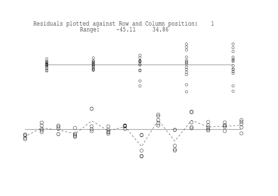
The residual plot from this analysis is presented in in the figure.

{Figure 2. Residual plots for the EXP variance model for the plant data. This suggests increasing variance over time. This can be modelled by using the EXPH model, which models Σ by Σ = D0.5CD0.5 where D is a diagonal matrix of variances and C is a correlation matrix with elements given by cij = φ|ti- tj|. The coding for this is
 y1 y3 y5 y7 y10 ~ Trait tmt Tr.tmt
 residual units.exph(Trait !COORD  1 3 5 7 10 )
Note that it is necessary to fix the scale parameter to 1 ( !SIGMAPAR) to ensure that the elements of D are identifiable. Abbreviated output from this analysis is
    1 LogL=-195.598     S2=  1.0000         60 df    :   1 components constrained
    2 LogL=-179.036     S2=  1.0000         60 df
    3 LogL=-175.483     S2=  1.0000         60 df
    4 LogL=-173.128     S2=  1.0000         60 df
    5 LogL=-171.980     S2=  1.0000         60 df
    6 LogL=-171.615     S2=  1.0000         60 df
    7 LogL=-171.527     S2=  1.0000         60 df
    8 LogL=-171.504     S2=  1.0000         60 df
    9 LogL=-171.498     S2=  1.0000         60 df
   10 LogL=-171.496     S2=  1.0000         60 df

          - - - Results from analysis of y1 y3 y5 y7 y10 - - -
 Akaike Information Criterion      354.99 (assuming 6 parameters).
 Bayesian Information Criterion    367.56

 Model_Term                             Sigma         Sigma   Sigma/SE   % C
 units.exph(Trait)               70 effects
 Trait                   EXP_P    1  0.906635      0.906635      21.79   0 P
 Trait                   EXP_V    1   60.6454       60.6454       2.14   0 P
 Trait                   EXP_V    2   73.3402       73.3402       1.98   0 P
 Trait                   EXP_V    3   308.295       308.295       2.23   0 P
 Trait                   EXP_V    4   434.744       434.744       2.53   0 P
 Trait                   EXP_V    5   381.287       381.287       2.75   0 P
 Covariance/Variance/Correlation Matrix  Residual
   60.50      0.8218      0.6753      0.5549      0.4134
   54.80       73.51      0.8218      0.6753      0.5030
   92.16       123.6       307.8      0.8218      0.6121
   89.92       120.6       300.4       434.0      0.7449
   62.74       84.15       209.6       302.8       380.7

                                    Wald F statistics
      Source of Variation                DF      F_inc
    8 Trait                               5     127.95
    1 tmt                                 1       0.00
    9 Tr.tmt                              4       4.75
The last two models we fit are the antedependence model of order 1
and the unstructured model. These require, as starting values the
lower triangle of the full variance matrix. We use the REML estimate
of Σ from the heterogeneous power model shown in the
previous output. The antedependence model models Σ by the
inverse cholesky decomposition
Σ-1 = UDU'
where D is a diagonal matrix and U is a unit upper
triangular matrix. For an antedependence model of order q, then
uij = 0 for j>i+q-1. The antedependence model of order 1 has 9
parameters for these data, 5 in D and 4 in U. The input is given by
y1 y3 y5 y7 y10 ~ Trait tmt Tr.tmtThe abbreviated output file isunits.ante(Trait)
  1 LogL=-171.501     S2=  1.0000         60 df
  2 LogL=-170.097     S2=  1.0000         60 df
  3 LogL=-166.085     S2=  1.0000         60 df
  4 LogL=-161.335     S2=  1.0000         60 df
  5 LogL=-160.407     S2=  1.0000         60 df
  6 LogL=-160.370     S2=  1.0000         60 df
  7 LogL=-160.369     S2=  1.0000         60 df

          - - - Results from analysis of y1 y3 y5 y7 y10 - - -
 Akaike Information Criterion      338.74 (assuming 9 parameters).
 Bayesian Information Criterion    357.59

 Model_Term                             Sigma         Sigma   Sigma/SE   % C
 units.ante(Trait)               70 effects
 Trait                 ANTE_U  1  1  0.268753E-01  0.268753E-01   2.44   0 P
 Trait                 ANTE_U  2  1 -0.628277     -0.628277      -2.56   0 P
 Trait                 ANTE_U  2  2  0.372717E-01  0.372717E-01   2.41   0 P
 Trait                 ANTE_U  3  2  -1.49128      -1.49128      -2.54  -1 P
 Trait                 ANTE_U  3  3  0.599625E-02  0.599625E-02   2.43   0 P
 Trait                 ANTE_U  4  3  -1.28095      -1.28095      -6.19   0 P
 Trait                 ANTE_U  4  4  0.789625E-02  0.789625E-02   2.44   0 P
 Trait                 ANTE_U  5  4 -0.967738     -0.967738     -15.40   0 P
 Trait                 ANTE_U  5  5  0.390634E-01  0.390634E-01   2.45   0 P
 Covariance/Variance/Correlation Matrix ANTE Residual
   37.19      0.5946      0.3536      0.3102      0.3028
   23.34       41.42      0.5946      0.5217      0.5092
   34.66       61.51       258.4      0.8774      0.8563
   44.38       78.77       330.9       550.4      0.9760
   42.94       76.21       320.1       532.5       540.8

                                   Wald F statistics
     Source of Variation           NumDF              F-inc
   8 Trait                             5             189.36
   1 tmt                               1               4.19
   9 Tr.tmt                            4               3.91
The iterative sequence converged and the antedependence parameter
estimates are printed columnwise by time,
the column of U and the element of D. I.e.
D = diag( 0.0269 0.0373 0.0060 0.0079 0.0391 ),
U =
| 1.0 | -0.6284 | 0 | 0 | 0 |
| 0 | 1 | -1.4911 | 0 | 0 |
| 0 | 0 | 1 | -1.2804 | 0 |
| 0 | 0 | 0 | 1 | -0.9678 |
| 0 | 0 | 0 | 0 | 1 . |
Finally the input and output files for the unstructured model are presented below. The REML estimate of Σ from the ANTE model is used to provide starting values.
y1 y3 y5 y7 y10 ~ Trait tmt Tr.tmtThe antedependence model of order 1 is clearly more parsimonious than the unstructured model. The next Table presents the incremental Wald tests for each of the variance models. There is a surprising level of discrepancy between models for the Wald tests. The main effect of treatment is significant for the uniform, power and antedependence models. Table Summary of Wald test for fixed effects for variance models fitted to the plant dataunits.us(Trait) 1 LogL=-160.368 S2= 1.0000 60 df 2 LogL=-159.027 S2= 1.0000 60 df 3 LogL=-158.247 S2= 1.0000 60 df 4 LogL=-158.040 S2= 1.0000 60 df 5 LogL=-158.036 S2= 1.0000 60 df - - - Results from analysis of y1 y3 y5 y7 y10 - - - Akaike Information Criterion 346.07 (assuming 15 parameters). Bayesian Information Criterion 377.49 Model_Term Sigma Sigma Sigma/SE % C units.us(Trait) 70 effects Trait US_V 1 1 37.2262 37.2262 2.45 0 P Trait US_C 2 1 23.3935 23.3935 1.77 0 P Trait US_V 2 2 41.5195 41.5195 2.45 0 P Trait US_C 3 1 51.6524 51.6524 1.61 0 P Trait US_C 3 2 61.9169 61.9169 1.78 0 P Trait US_V 3 3 259.121 259.121 2.45 0 P Trait US_C 4 1 70.8113 70.8113 1.54 0 P Trait US_C 4 2 57.6146 57.6146 1.23 0 P Trait US_C 4 3 331.807 331.807 2.29 0 P Trait US_V 4 4 551.507 551.507 2.45 0 P Trait US_C 5 1 73.7857 73.7857 1.60 0 P Trait US_C 5 2 62.5691 62.5691 1.33 0 P Trait US_C 5 3 330.851 330.851 2.29 0 P Trait US_C 5 4 533.756 533.756 2.42 0 P Trait US_V 5 5 542.175 542.175 2.45 0 P Covariance/Variance/Correlation Matrix US Residual 37.23 0.5950 0.5259 0.4942 0.5194 23.39 41.52 0.5969 0.3807 0.4170 51.65 61.92 259.1 0.8777 0.8827 70.81 57.61 331.8 551.5 0.9761 73.79 62.57 330.9 533.8 542.2 Wald F statistics Source of Variation NumDF F-inc 8 Trait 5 196.02 1 tmt 1 1.72 9 Tr.tmt 4 4.46
| treatment | treatment.time | |
| model | (df=1) | (df=4) |
| Uniform | 9.41 | 5.10 |
| Power | 6.86 | 6.13 |
| Heterogeneous power | 0.00 | 4.81 |
| Antedependence (order 1) | 4.14 | 3.96 |
| Unstructured | 1.71 | 4.46 |
